Matrix Multiplication, From Definition to Cache Lines

Every model I have shipped — every transformer layer, every value head, every speech encoder — spends most of its FLOPs inside one operation. For $A \in \R^{m \times k}$ and $B \in \R^{k \times n}$, the product $C = AB$ is defined entrywise:

$$c_{ij} = \sum_{p=1}^{k} a_{ip}\, b_{pj}, \qquad 1 \le i \le m,\ \; 1 \le j \le n.$$

That is $mnk$ multiply–adds — $2mnk$ floating-point operations — and the definition translates directly into the first matmul everyone writes. The definition is three loops. The performance is a memory story, and this post walks it down to the cache line.

Three ways to spend 268 million FLOPs

At $m = n = k = 512$ the product costs $2 \cdot 512^3 \approx 2.7 \times 10^8$ FLOPs. Here is the definition, verbatim — this exact function is what the benchmark script times:

def matmul_naive(A, B, n):
    C = [[0.0] * n for _ in range(n)]
    for i in range(n):
        for j in range(n):
            acc = 0.0
            for p in range(n):
                acc += A[i][p] * B[p][j]
            C[i][j] = acc
    return C

On my desktop this takes 9.3 s over Python lists. The obvious “optimization” — the same three loops over NumPy arrays, indexed one scalar at a time (A[i, p] * B[p, j]) — takes 41.9 s, 4.5× as long as plain lists. And A @ B, which dispatches to OpenBLAS, takes 5.1 ms on a single thread. Same matrices, same 268 million FLOPs, answers identical to within $2.3 \times 10^{-13}$:

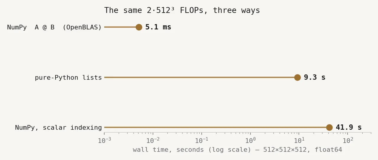
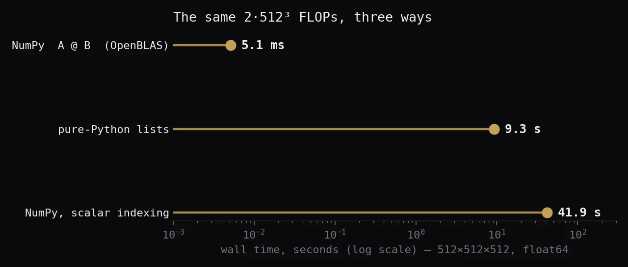
Two things in that chart deserve an explanation. The scandal — NumPy losing to plain lists by 4.5× — is the cheap one: every A[i, p] crosses the C-API boundary and boxes a fresh Python float object, about 120 ns of overhead per element access, 268 million times. NumPy’s contract is whole-array operations; index it like a list and you pay for the machinery without ever engaging it.

The interesting number is the other one: 1800× between the honest loops and A @ B, with OpenBLAS performing exactly the $2mnk$ FLOPs the definition demands, in the same double precision. The interpreter accounts for maybe two orders of magnitude of that — a compiled -O3 version of the same triple loop typically lands at one or two GFLOP/s on this class of core. The rest, the factor of thirty-odd that survives compilation, is memory.

Benchmark environment

Intel i7-6700K (Skylake, 4 cores / 8 threads, 4.0 GHz base / 4.2 GHz single-core turbo), caches 32 KB L1d + 256 KB L2 per core, 8 MB shared L3, dual-channel DDR4. Python 3.11.7, NumPy 2.4.2 linked against scipy-openblas, float64 throughout. BLAS pinned to one thread with OPENBLAS_NUM_THREADS=1 except in the multithreaded runs at the end. The two slow loops run once; every other timing is best-of-5 with a fixed seed. Results cross-checked against A @ B: max abs deviation ≈ 2.3 × 10⁻¹³.

The 64-byte truth

A CPU never reads one float64 from memory. It reads a cache line — 64 bytes, eight doubles — and keeps it in a hierarchy of caches: on this machine 32 KB of L1d per core, 256 KB of L2, 8 MB of L3 shared by all cores. A load that hits L1 costs ~4 cycles; a trip to DRAM costs a couple hundred. Everything about fast numerical code follows from one rule: when you pull a line, use what is on it — and reuse it before it is evicted.

NumPy stores matrices row-major (C order): row $i$ is contiguous, and element $b_{pj}$ lives 8 bytes after $b_{p,j-1}$ but a full row-length after $b_{p-1,j}$. Now look at the inner loop of the definition: it walks A[i][p] along a row — sequential, eight useful doubles per fetched line, a pattern the hardware prefetcher recognizes and runs ahead of — and B[p][j] down a column, jumping 4 KB per step. Every step of that walk opens a different cache line and a different memory page; one pass down a column touches 512 lines (32 KB of traffic for 4 KB of useful data), and the prefetcher sees nothing it can work with.

The effect is easy to isolate without any matmul. Take one 8192×8192 matrix — 537 MB, far bigger than any cache — and sum it twice, once walking rows, once walking columns:

M = rng.standard_normal((8192, 8192))

s = 0.0
for i in range(8192): s += M[i, :].sum()   # along rows:    44 ms

s = 0.0
for j in range(8192): s += M[:, j].sum()   # down columns: 597 ms

Same bytes, same additions, 13.6× apart. The row pass streams whole cache lines behind the prefetcher. The column pass uses one double per line it opens on that pass, and its 64 KB stride touches 8192 distinct memory pages per column — far beyond what the TLB can hold, so accesses pay for page walks on top of cache misses. (Neighbouring columns do salvage the other seven doubles of each line from L3 later — which is why the penalty is 13.6× and not worse.) The row pass moves 537 MB in 44 ms — about 12.2 GB/s, this core’s practical read bandwidth. Keep that number.

Arithmetic intensity, or why the naive loop cannot be fast

A core is bounded by two ceilings: how fast it computes and how fast it is fed. This one, at 4.2 GHz with two 256-bit FMA ports, peaks at

$$4.2\ \text{GHz} \times 2\ \tfrac{\text{FMA}}{\text{cycle}} \times 4\ \tfrac{\text{doubles}}{\text{FMA}} \times 2\ \tfrac{\text{FLOP}}{\text{double}} \;\approx\; 67\ \tfrac{\text{GFLOP}}{\text{s}}$$

in double precision — but sustains only ~12.2 GB/s of reads. Which ceiling applies is decided by arithmetic intensity: FLOPs performed per byte moved.

The naive loop, run at sizes where the operands have outgrown the caches, streams both operands through the core once per use — two 8-byte reads per multiply–add, an intensity of $q = \tfrac{2\ \text{FLOP}}{16\ \text{B}} = 0.125$. At 12.2 GB/s that caps even a perfectly vectorized loop with this access pattern at about $0.125 \times 12.2 \approx 1.5$ GFLOP/s — over forty times below the compute peak, before a single cycle of interpreter overhead is charged. That is the ceiling compilation cannot lift: the loop itself is memory-bound by construction.

To go fast we do not need fewer FLOPs. We need more FLOPs per byte.

Blocking: the √M idea

The fix is decades old and still carries every BLAS and every GPU matmul kernel: tile the problem so a small working set lives in cache and is reused before eviction.

Cut the matrices into $b \times b$ tiles and accumulate each tile of $C$ as a sum of little tile products:

for i0 in range(0, n, b):
    for j0 in range(0, n, b):
        # this C tile is reused across the entire p-loop
        for p0 in range(0, n, b):
            C[i0:i0+b, j0:j0+b] += A[i0:i0+b, p0:p0+b] @ B[p0:p0+b, j0:j0+b]

One step of the inner loop touches three $b \times b$ tiles — $3b^2 \times 8$ bytes — and performs $2b^3$ FLOPs on them:

$$q(b) \;=\; \frac{2b^3}{24\, b^2}\ \tfrac{\text{FLOP}}{\text{B}} \;=\; \frac{b}{12}\ \tfrac{\text{FLOP}}{\text{B}},$$

an intensity that grows with the tile size. To lift this core from memory-bound to compute-bound we need $q \gtrsim 67 / 12.2 \approx 5.5$, i.e. $b$ of about seventy — and three 70×70 float64 tiles occupy 118 KB, a comfortable fit in the 256 KB L2. That is the entire trick, and it is why cache capacity $M$ appears under a square root all over this literature: tiles of side $b \sim \sqrt{M/3}$ cut total traffic from the naive $\mathcal{O}(n^3)$ words down to

$$\mathcal{O}\!\left(\frac{n^3}{\sqrt{M}}\right),$$

which Hong and Kung proved in 1981 is asymptotically optimal for any schedule of the classical algorithm. Bigger cache, less traffic — by the square root.

What a real BLAS adds

OpenBLAS is this idea executed with obsession: tile sizes tuned per cache level, operand packing (each tile is copied into a contiguous aligned buffer, so even the walk down $B$ becomes sequential line-by-line streaming), and an innermost register microkernel that pins a small block of $C$ in vector registers while FMAs stream over it. The payoff fits in one chart:

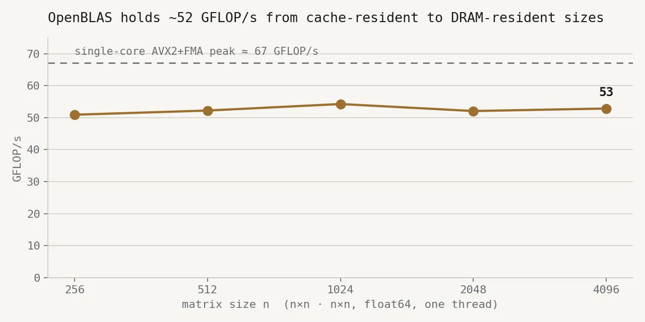
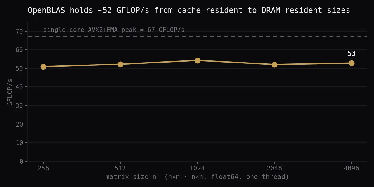
Flat. From $n = 256$, where all three matrices fit in the L3, to $n = 4096$, where 268 MB of operands (400 MB counting the output) live in DRAM, throughput holds at 51–54 GFLOP/s — 79% of the theoretical single-core peak at the largest size — because blocking makes the FLOP-per-byte ratio a property of the tile, not of the problem size. The definitional loop gets slower per FLOP each time the matrices outgrow another cache level; the blocked loop does not care.

Two footnotes from the same machine, both measured. First, parallelism: pinned to the four physical cores, $n = 4096$ runs at 179 GFLOP/s — a 3.4× speedup, the shortfall from 4× being mostly all-core turbo running below single-core turbo, plus some sharing of the L3 and DRAM channels. Left at its default, OpenBLAS spawns eight threads on this machine — one per hyperthread — and drops to 118 GFLOP/s: two SMT siblings share one physical core’s FMA pipes, so the extra threads add scheduling overhead and no compute. Count physical cores. Second, 79% of peak is where a mature BLAS lands on this microarchitecture in float64 — the missing fifth goes to packing traffic, tile edges, and loop bookkeeping. Nobody gets 100%.

The same idea, all the way up

Swap “L2” for “shared memory” and this becomes a CUDA lecture: a GPU matmul kernel stages tiles of $A$ and $B$ in each SM’s shared memory, syncs, multiplies, advances — the identical $\sqrt{M}$ argument, executed by thousands of threads. Tensor cores move the tile into the datapath itself: a warp feeds fixed-size fragments and the hardware performs the small dense product as single instructions. One level higher, an attention layer or an MLP block is a batch of these products — which is why arithmetic intensity, usually rephrased as FLOPs per byte of weights, still decides whether a transformer is compute-bound or bandwidth-bound on an H100.

The definition is three loops, essentially unchanged since Binet wrote the row-by-column rule down in 1812. Everything between 9.3 seconds and 5.1 milliseconds is knowing where your cache lines are.

Reproduce it

matmul_bench.py — ~130 lines of stdlib-plus-NumPy Python: the two slow loops (single runs), the BLAS size sweep and the traversal demo (best-of-5), and the multithreaded runs, all with a fixed seed. It times the exact functions shown above. Absolute numbers will differ on your machine; the ratios will not. Run it before believing me.