NumPy Cheatsheet
All examples from DataCamp’s NumPy cheat sheet, run in NumPy 2.4. Each one has its code and a picture. The pictures are drawn by running that same code, so they show what NumPy actually returns.
How to read the pictures: a filled cell is one the operation selects, reads or produces. A thick outline marks cells a step has just written. Dashed, faded cells are values NumPy repeats by broadcasting. Small numbers in a cell’s corner give element order. Grey numbers along the edges are indices, counted from zero.
Where the original sheet fails or is wrong in NumPy 2, the example is fixed and the text says what changed. The examples use these arrays:
import numpy as np

a = np.array([1, 2, 3])
b = np.array([(1.5, 2, 3), (4, 5, 6)], dtype=float)
c = np.array([[(1.5, 2, 3), (4, 5, 6)], [(3, 2, 1), (4, 5, 6)]], dtype=float)
d = np.arange(10, 25, 5)
e = np.full((2, 2), 7)
f = np.eye(2)
g = a - b
Creating arrays
1D, 2D, 3D
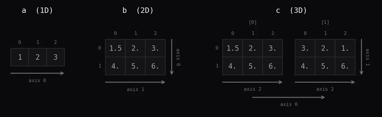
Axes are numbered from the outside in, and axis 0 is the first index. In a 2D array axis 0 runs over the rows. In a 3D array it runs over the blocks.
a = np.array([1, 2, 3])
b = np.array([(1.5, 2, 3), (4, 5, 6)], dtype=float)
c = np.array([[(1.5, 2, 3), (4, 5, 6)], [(3, 2, 1), (4, 5, 6)]], dtype=float)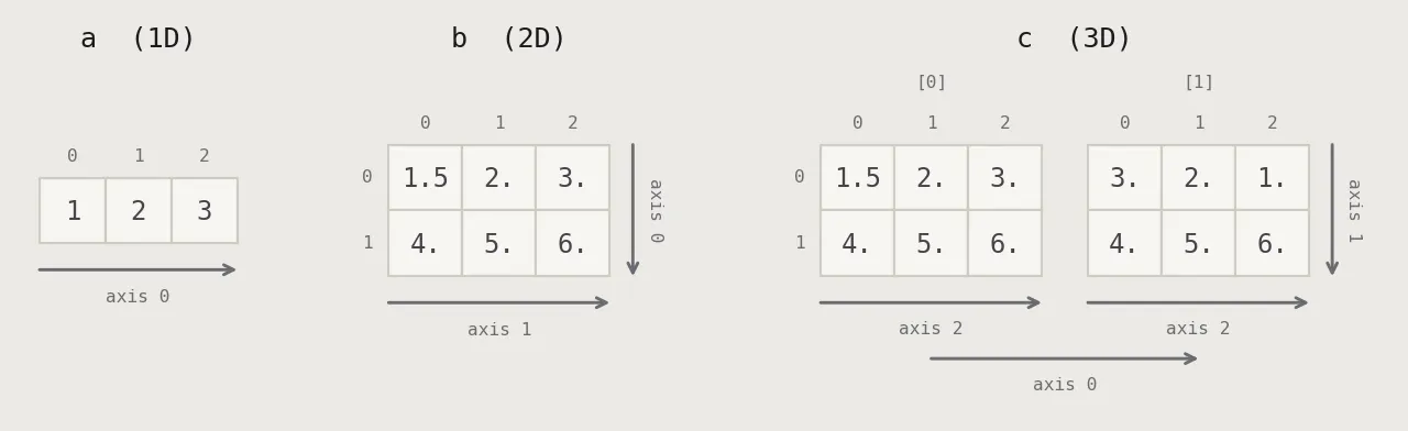
Initial placeholders
np.zeros
A new array of the given shape filled with 0. The default type is float64, hence 0..
np.zeros((3, 4))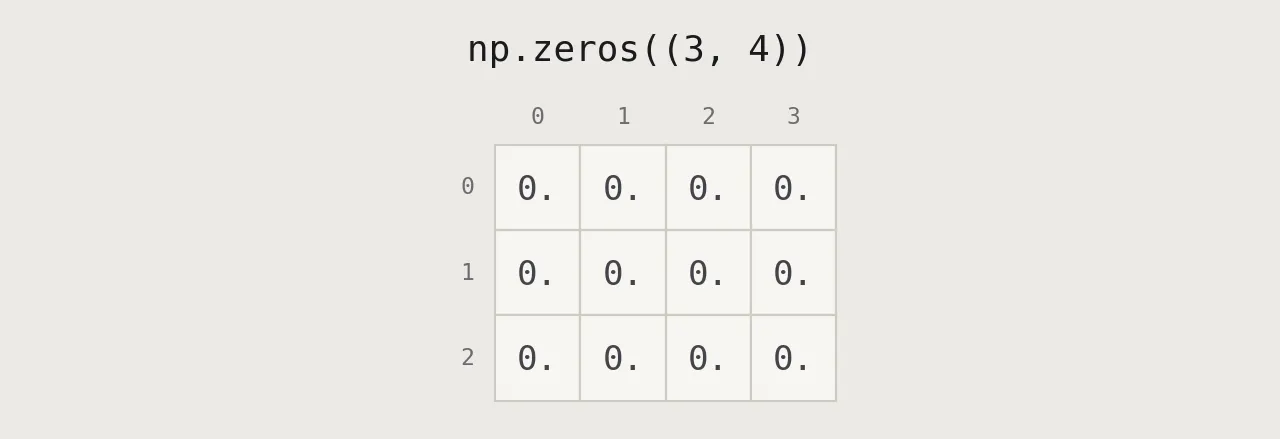

np.ones
Ones, here as 16-bit integers. Shape (2, 3, 4) means 2 blocks of 3 rows and 4 columns.
np.ones((2, 3, 4), dtype=np.int16)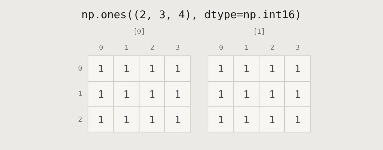
np.arange
Values from start up to stop with a fixed step. Stop itself is excluded, so 25 is not in the result.
d = np.arange(10, 25, 5)

np.linspace
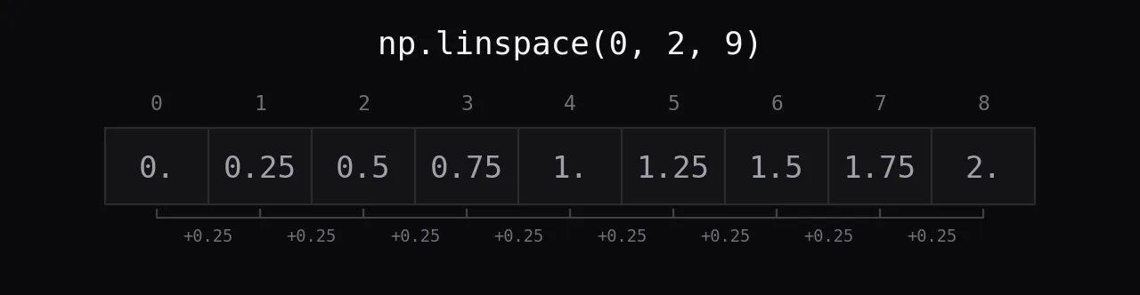
A fixed number of evenly spaced values, both ends included. 9 samples from 0 to 2 give a step of 0.25.
np.linspace(0, 2, 9)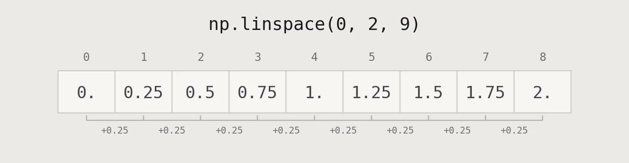
np.full
Any shape, filled with one constant.
e = np.full((2, 2), 7)

np.eye
An identity matrix: ones on the diagonal, zeros elsewhere.
f = np.eye(2)

np.random.random
Uniform random floats from 0 (included) to 1 (excluded). New code usually writes np.random.default_rng().random((2, 2)).
np.random.random((2, 2))

np.empty
Allocates memory without initialising it. The values are whatever was in that memory before, so fill the array before you read it.
np.empty((3, 2))

I/O
np.save, np.load
np.save writes one array in NumPy’s binary .npy format and adds the extension itself. The file holds a small header with the type and shape, then the raw bytes: 3 int64 values take 24 bytes.
np.save('my_array', a)
np.load('my_array.npy')

np.savez
Several arrays in one uncompressed .npz archive. Arrays passed by position are named arr_0, arr_1 and so on; pass keywords, as in np.savez('array.npz', a=a, b=b), to choose the names. np.savez_compressed compresses.
np.savez('array.npz', a, b)
np.load('array.npz')['arr_1']

np.savetxt, np.loadtxt
Plain text, one row per line. The default format is %.18e, so every number is written as a float and loadtxt reads floats back. Pass fmt='%d' to write integers.
np.savetxt('myarray.txt', a, delimiter=' ')
np.loadtxt('myarray.txt')

np.genfromtxt
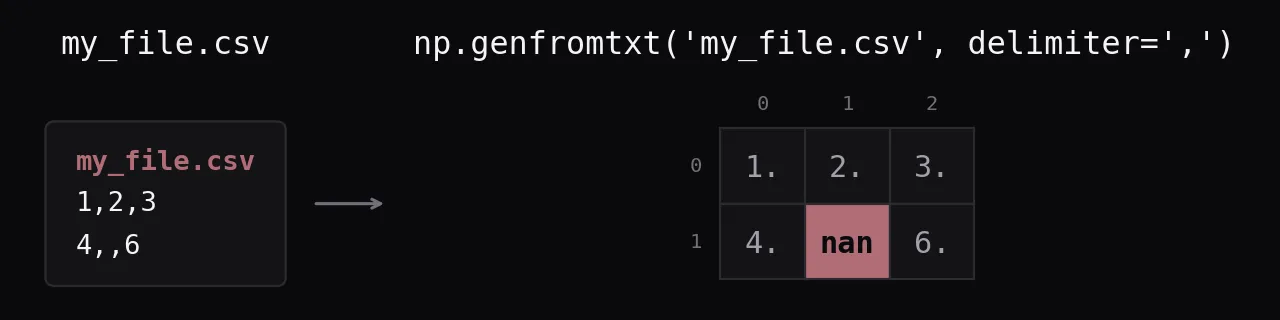
Like loadtxt, but it copes with missing values: the empty field becomes nan.
np.genfromtxt('my_file.csv', delimiter=',')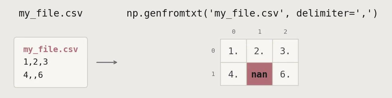
Data types
dtypes
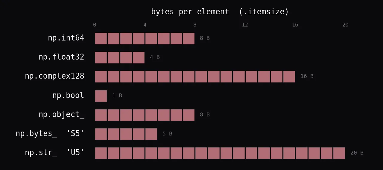
A type fixes how many bytes one element takes. Several names on the original sheet were removed in NumPy 2. np.complex, np.object, np.string_ and np.unicode_ are now np.complex128, np.object_, np.bytes_ and np.str_. The sheet also calls float32 double precision, but it is single precision; double is float64. An object array stores 8-byte pointers, and a unicode string uses 4 bytes per character.
np.int64       # signed 64-bit integer
np.float32     # single-precision float
np.complex128  # complex number, two float64
np.bool        # True / False
np.object_     # any Python object
np.bytes_      # fixed-length byte string, e.g. 'S5'
np.str_        # fixed-length unicode string, e.g. 'U5'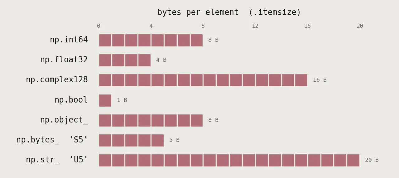
Inspecting your array
a.shape
The size along each axis, as a tuple. A 1D array gives a one-element tuple.
a.shape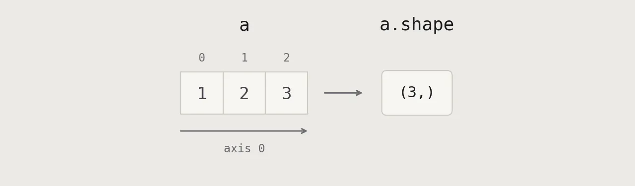

len
len counts only the first axis, so for a 2D array it gives the number of rows, not the number of elements.
len(b) # len(a) is 3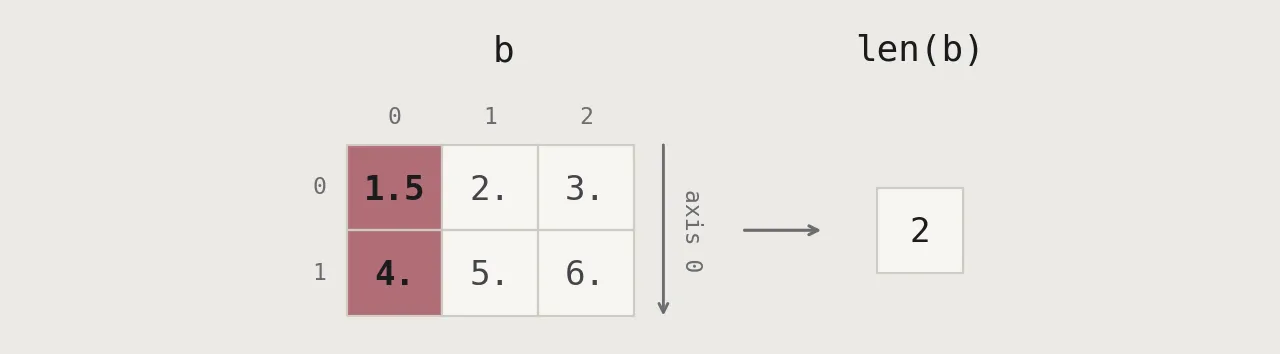
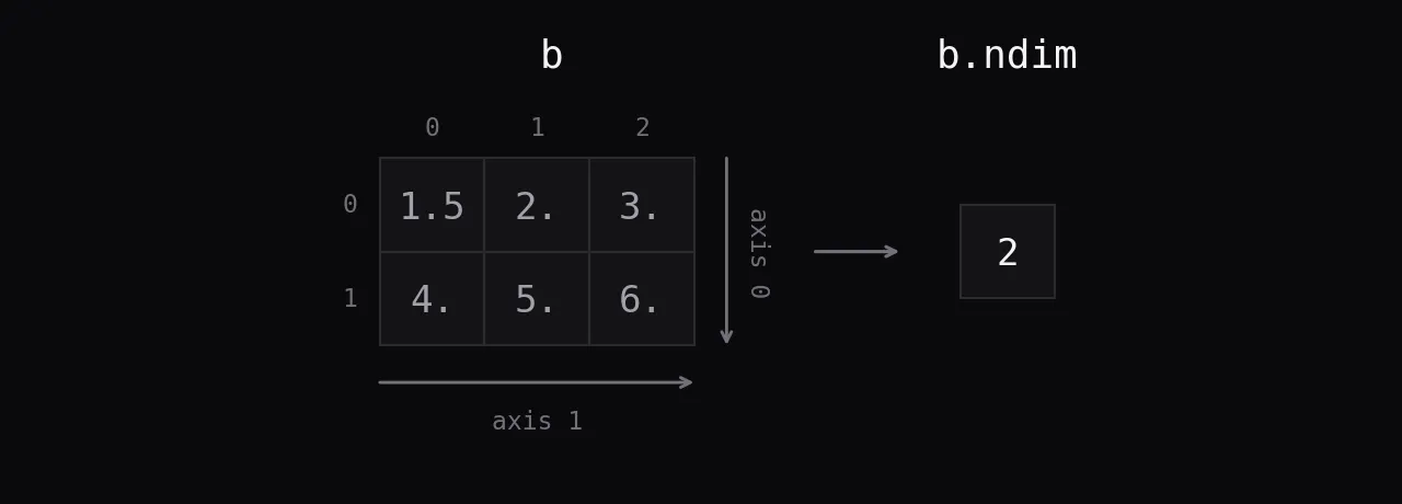
b.ndim
The number of axes.
b.ndim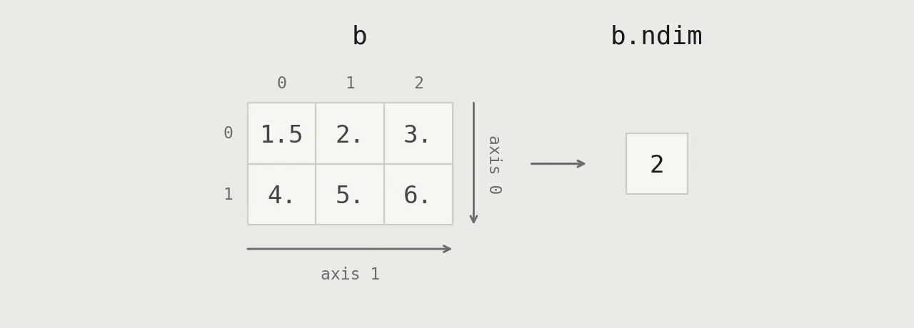
e.size
The total number of elements, the product of the shape.
e.size

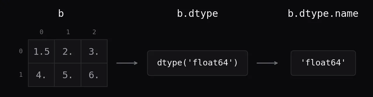
b.dtype
The element type, as a dtype object and as its name.
b.dtype
b.dtype.name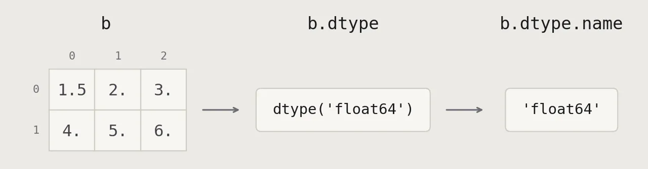
b.astype
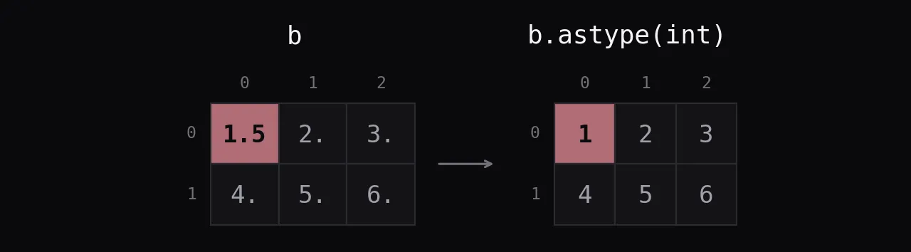
Converts to another type and returns a copy. Float to int truncates toward zero, so 1.5 becomes 1.
b.astype(int)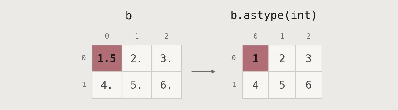
Asking for help
np.info
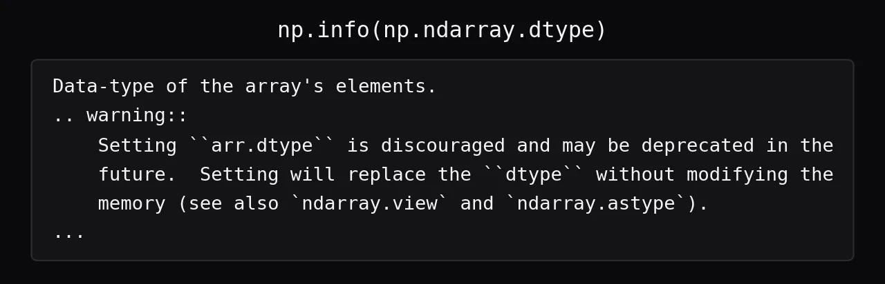
Prints the documentation of any NumPy object. help() works too.
np.info(np.ndarray.dtype)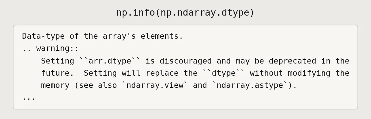
Arithmetic
a - b
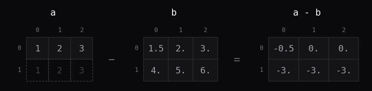
Element by element. a has shape (3,) and b has shape (2, 3), so NumPy broadcasts a over every row of b (the dashed row). The function form is the same operation.
g = a - b
np.subtract(a, b)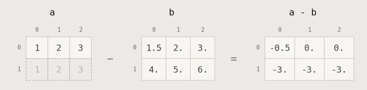
b + a
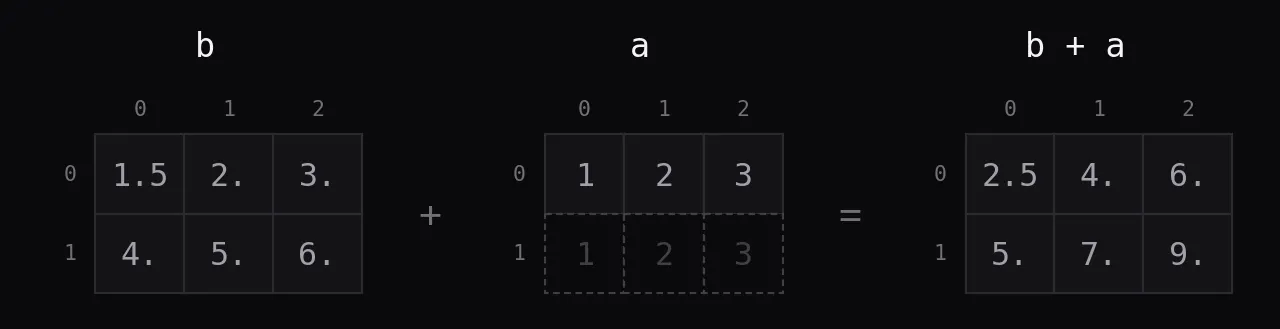
Addition, broadcast the same way. The order of the operands does not matter for broadcasting.
b + a
np.add(b, a)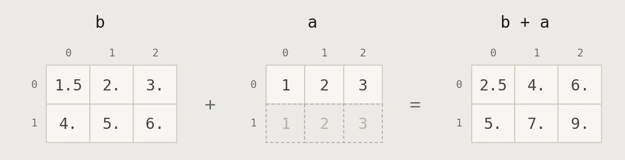
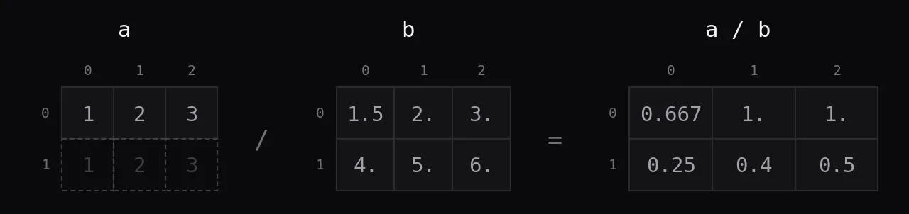
a / b
/ always returns floats, even for two integer arrays. // is integer division.
a / b
np.divide(a, b)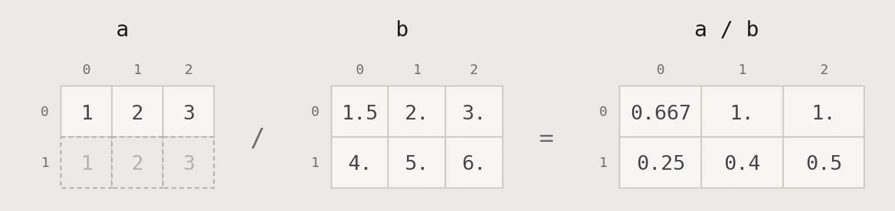
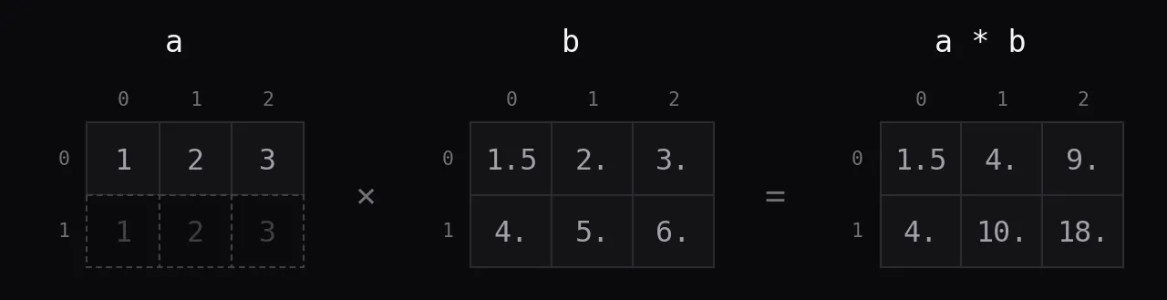
a * b
* multiplies element by element. It is not the matrix product; that is dot or @, below.
a * b
np.multiply(a, b)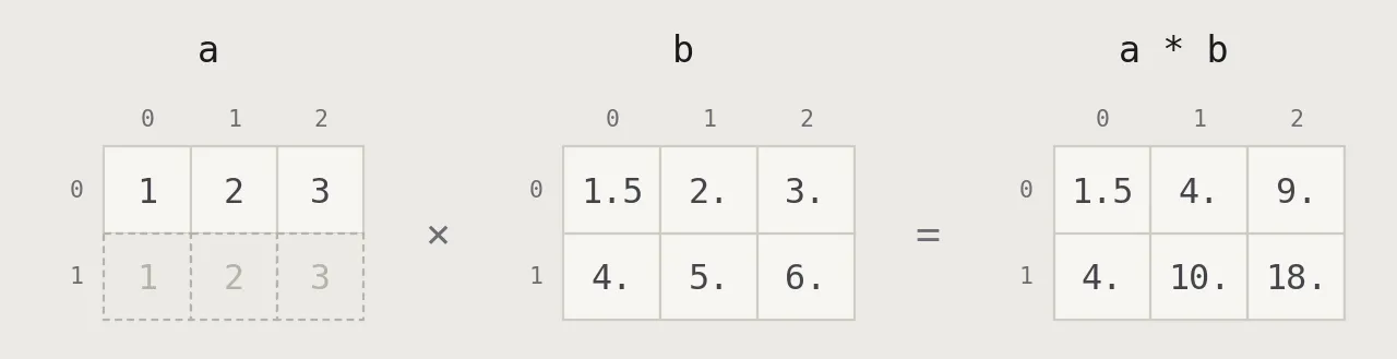
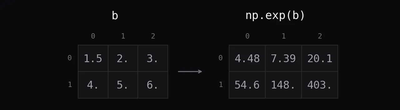
np.exp
Element-wise math functions keep the shape. This one is e to the power of each element.
np.exp(b)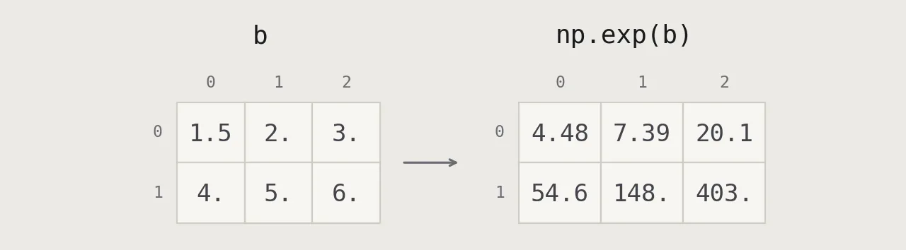
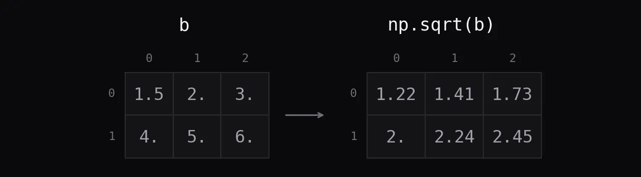
np.sqrt
Square root of each element.
np.sqrt(b)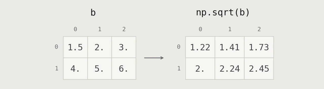
np.sin
Sine of each element, in radians.
np.sin(a)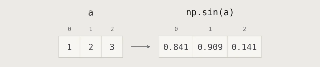

np.cos
Cosine of each element, in radians.
np.cos(b)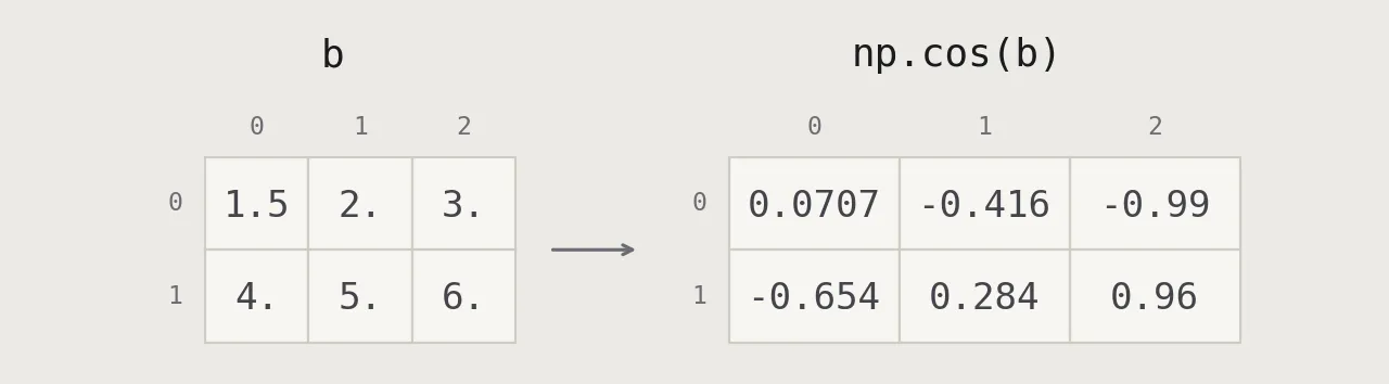
np.log
Natural logarithm of each element: log(1) is 0. np.log10 and np.log2 are the other bases.
np.log(a)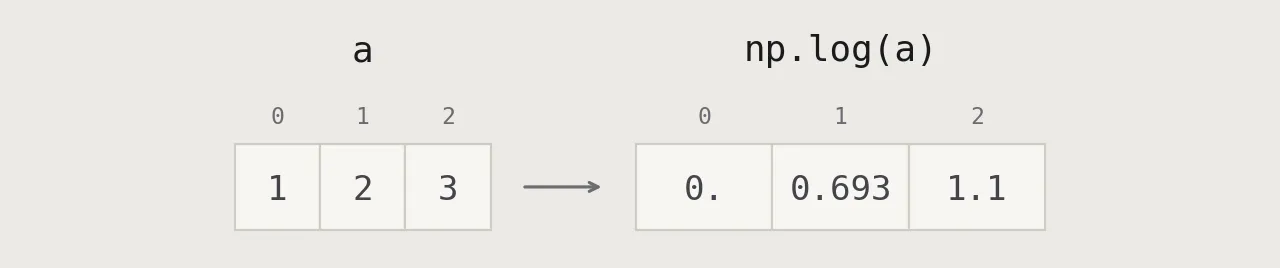

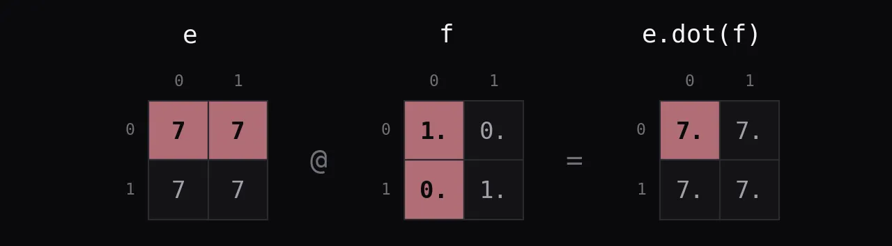
e.dot(f)
The matrix product: each result cell is a row of e times a column of f, summed. f is the identity, so the result equals e.
e.dot(f)
e @ f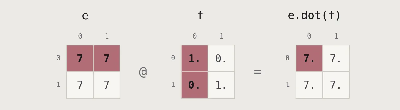
Comparison
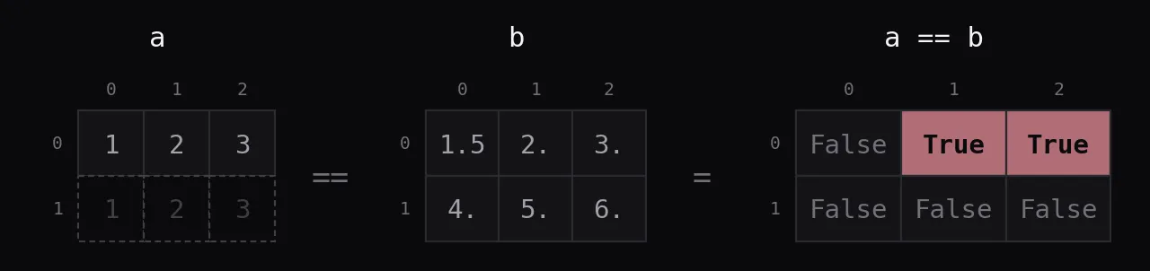
a == b
Element-wise comparison gives a bool array and broadcasts like arithmetic.
a == b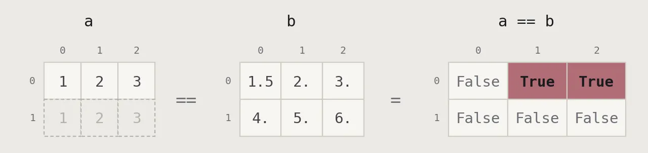
a < 2
Comparing with a number compares every element with it.
a < 2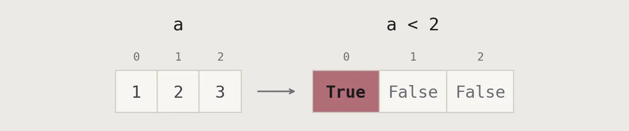

np.array_equal
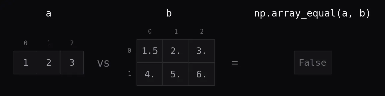
One bool for the whole array: True only if the shapes and all the values match. Here the shapes differ.
np.array_equal(a, b)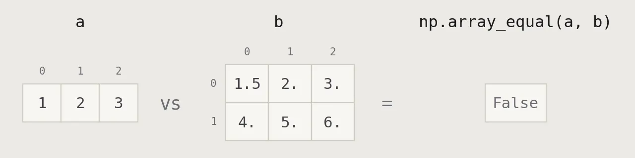
Aggregate functions
a.sum
Adds up all elements.
a.sum()

a.min
The smallest element. a.argmin() gives its index.
a.min()

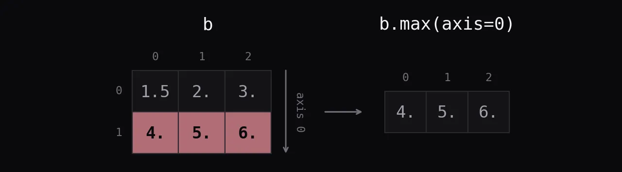
b.max(axis=0)
With axis=0 the reduction runs along axis 0, down the rows, so each column gives one value. The sheet says ‘of an array row’, but for axis=0 it is the maximum of each column.
b.max(axis=0)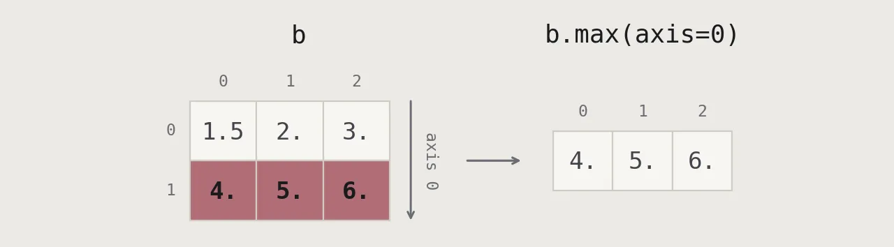
b.cumsum(axis=1)
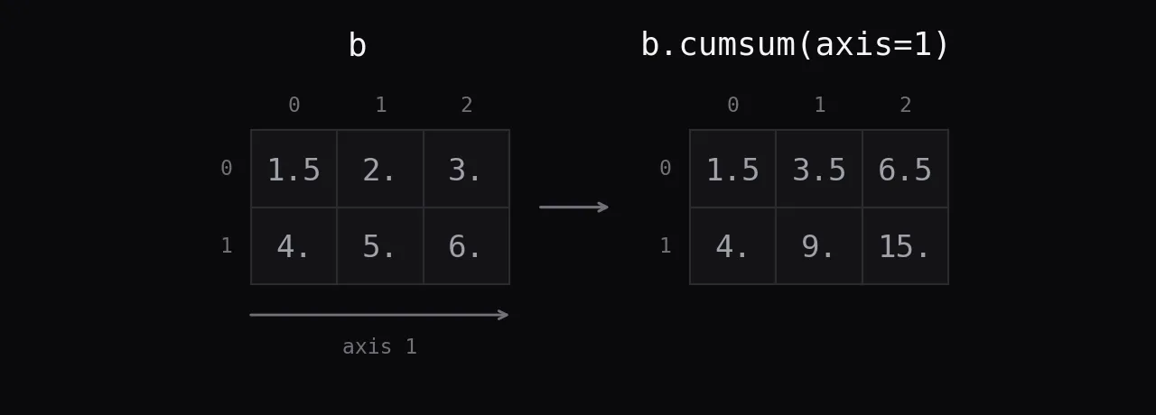
A running sum along each row. The shape stays the same.
b.cumsum(axis=1)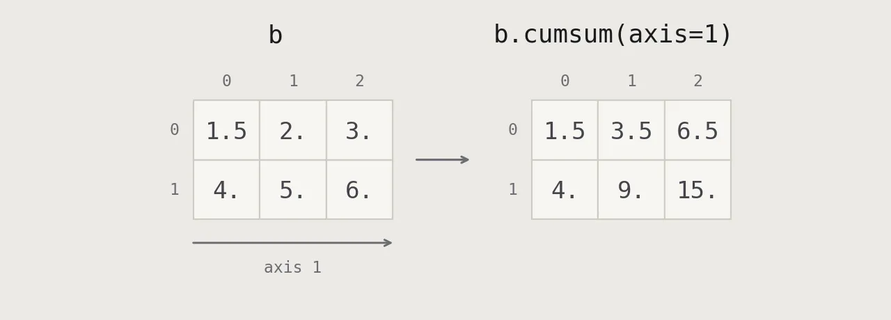
a.mean
The arithmetic mean of all elements.
a.mean()

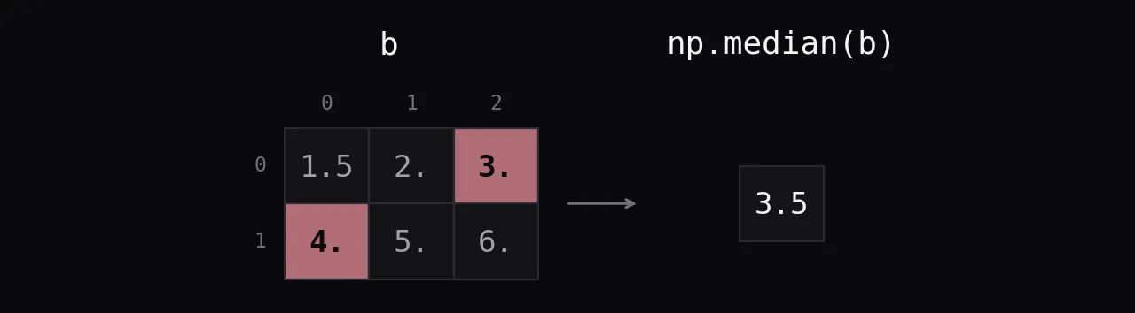
np.median
There is no b.median() method, so the sheet’s line raises AttributeError. Use np.median. With six values the median is the mean of the middle two, 3 and 4.
np.median(b)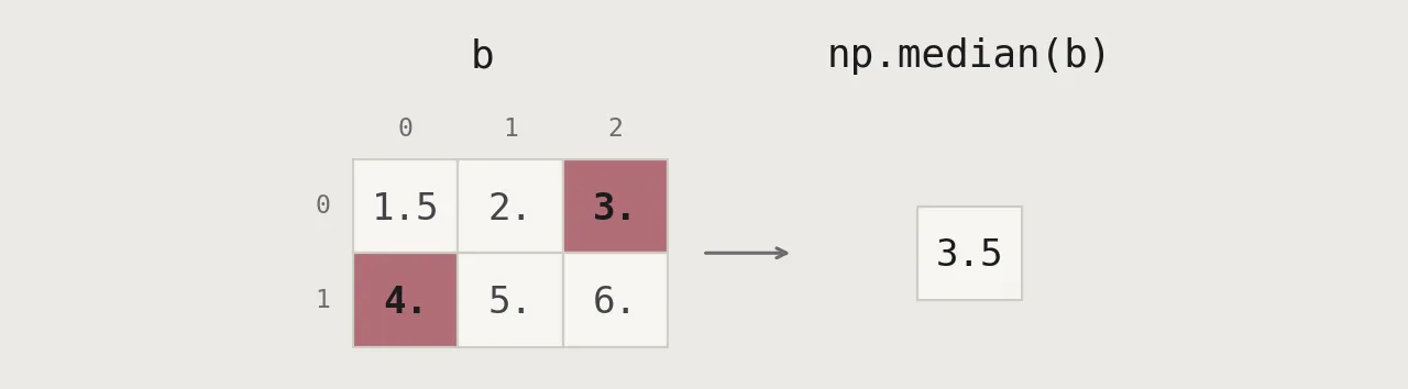
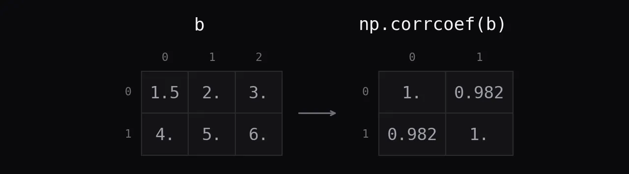
np.corrcoef
There is no a.corrcoef() method either. np.corrcoef treats each row as a variable and returns their correlation matrix. The two rows of b are almost perfectly correlated.
np.corrcoef(b)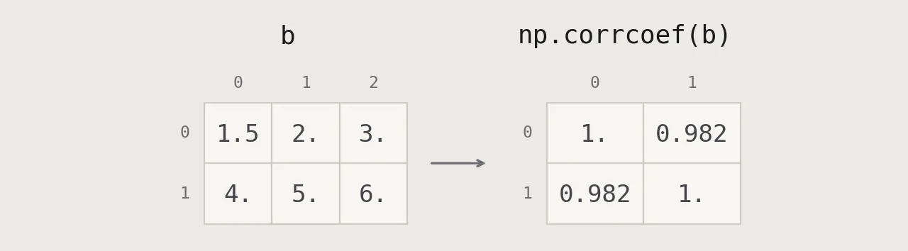
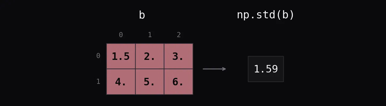
np.std
The standard deviation of all elements. By default it is the population version (ddof=0); pass ddof=1 for the sample version.
np.std(b)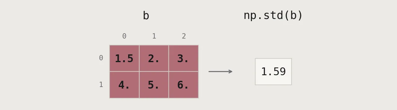
Copying arrays
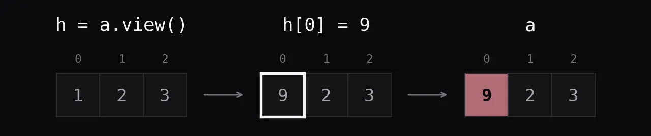
a.view
A view shares memory with the original, so writing through h changes a too.
h = a.view()
h[0] = 9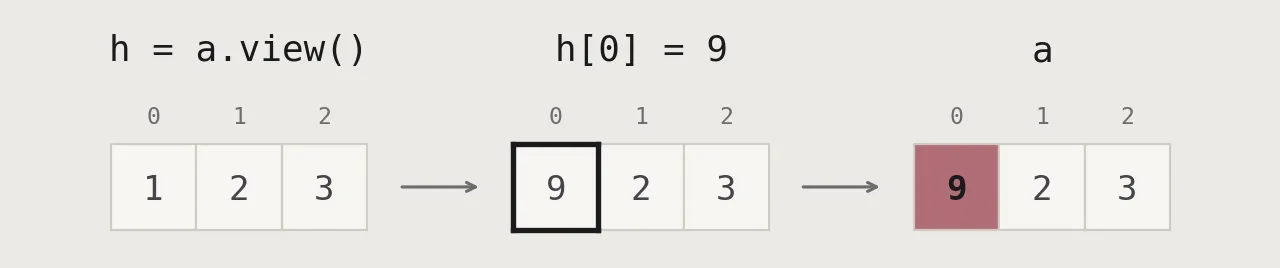
a.copy
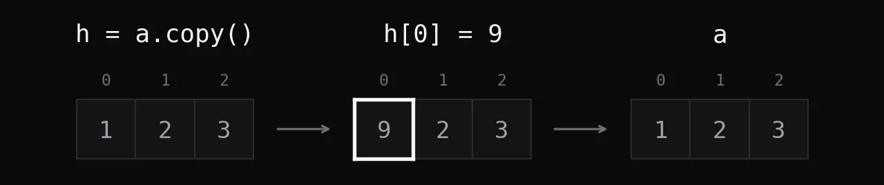
a.copy() and np.copy(a) both make an independent copy, so a stays unchanged.
h = a.copy()    # or np.copy(a)
h[0] = 9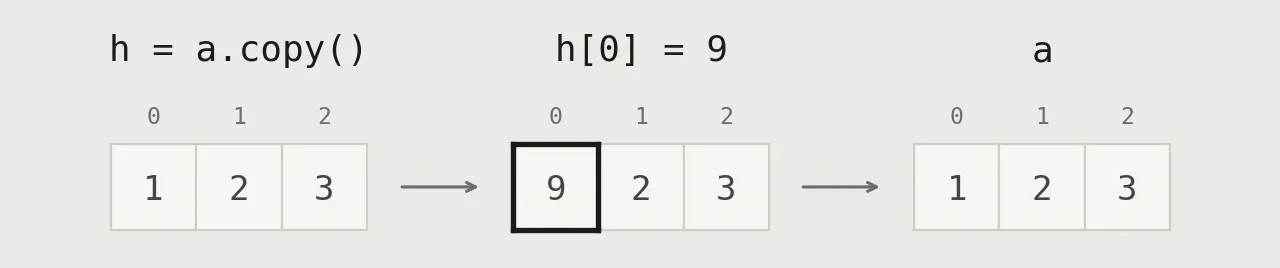
Sorting arrays
x.sort
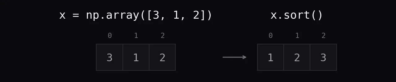
Sorts in place and returns None; np.sort(x) returns a sorted copy instead. The sheet’s a is already sorted, so this example uses x.
x = np.array([3, 1, 2])
x.sort()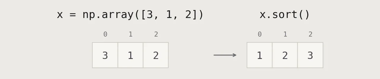
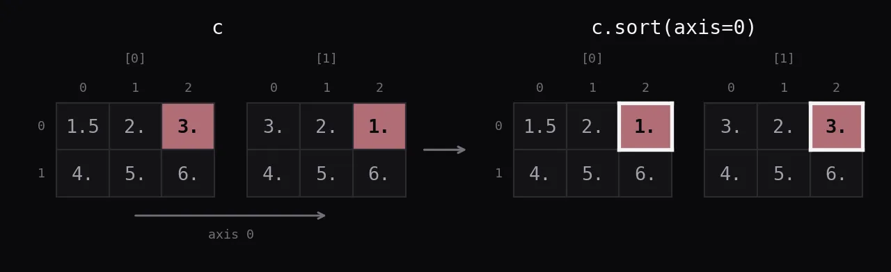
c.sort(axis=0)
Sorts along axis 0: each position is sorted across the two blocks. Only the 3 and the 1 in the corner are out of order, so only they swap.
c.sort(axis=0)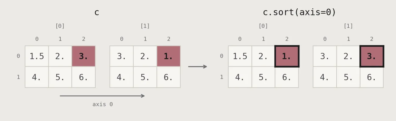
Subsetting, slicing, indexing
a[2]
The element at index 2.
a[2]

b[1, 2]
Row 1, column 2. The same as b[1][2], but one indexing step instead of two.
b[1, 2]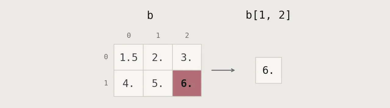

a[0:2]
Start is included, stop is excluded: indices 0 and 1.
a[0:2]

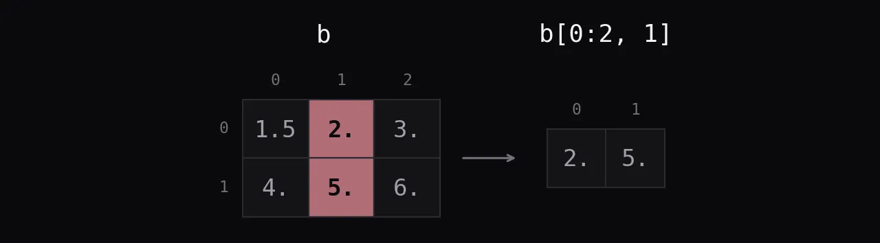
b[0:2, 1]
Rows 0 and 1 of column 1. A single index drops its axis, so the result is 1D.
b[0:2, 1]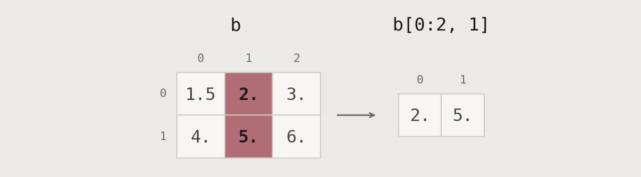
b[:1]
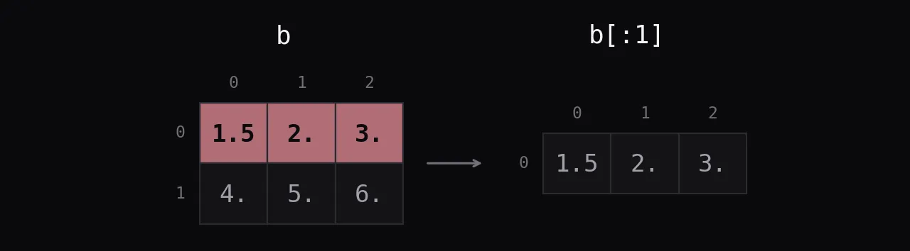
A slice keeps its axis: b[:1] is 2D with one row, while b[0] would be 1D. The same as b[0:1, :].
b[:1]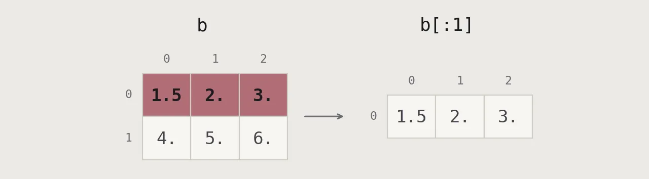
c[1, …]
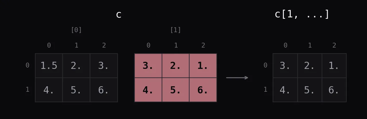
... stands for as many : as needed, so c[1, ...] is c[1, :, :], the second block. The sheet prints it with one bracket too many; the result is 2D.
c[1, ...]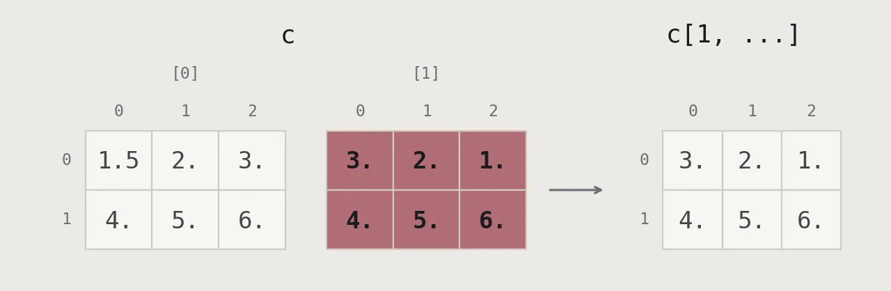
a[::-1]
A negative step walks backwards. The small numbers show where each element came from. The result is a view, not a copy.
a[::-1]

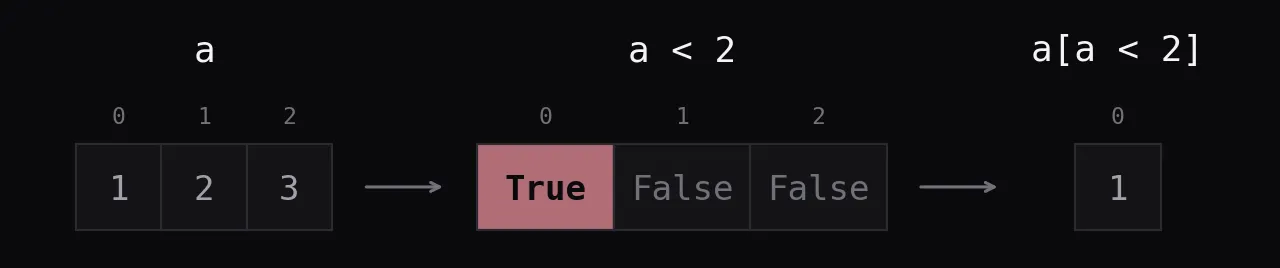
a[a < 2]
A bool array used as an index keeps the elements where it is True. The result is always 1D and always a copy.
a[a < 2]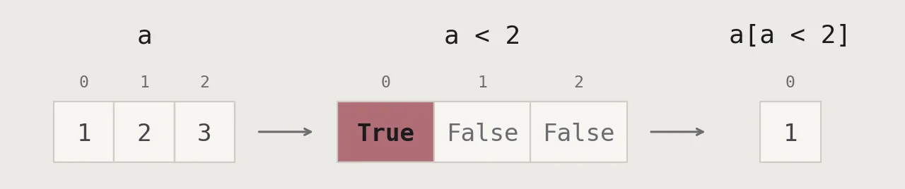
b[[1, 0, 1, 0], [0, 1, 2, 0]]
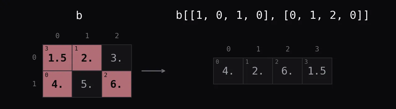
Two index lists pair up into (1, 0), (0, 1), (1, 2) and (0, 0). The small numbers show the order. Fancy indexing returns a copy.
b[[1, 0, 1, 0], [0, 1, 2, 0]]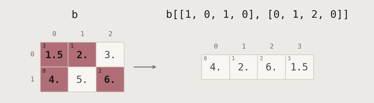
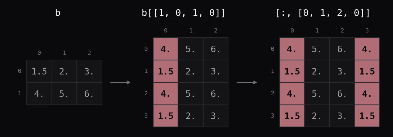
b[[1, 0, 1, 0]][:, [0, 1, 2, 0]]
First rows 1, 0, 1, 0, then columns 0, 1, 2, 0 of that result: a 4x4 grid with repeated rows and columns. b[np.ix_([1, 0, 1, 0], [0, 1, 2, 0])] does it in one step.
b[[1, 0, 1, 0]][:, [0, 1, 2, 0]]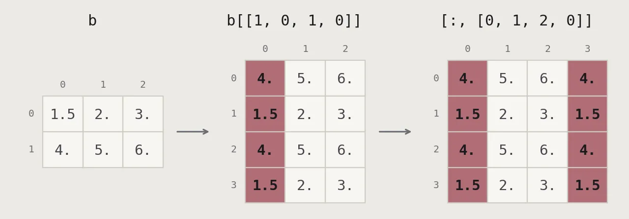
a[1:3] = 1
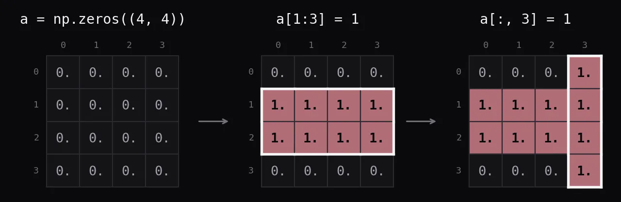
Not on the sheet: assigning through slices. a[1:3] is short for a[1:3, :], and the single number on the right is broadcast to every selected cell. Rows that are not next to each other take a list: a[[0, 3]] = 1.
a = np.zeros((4, 4))
a[1:3] = 1     # rows 1 and 2
a[:, 3] = 1    # column 3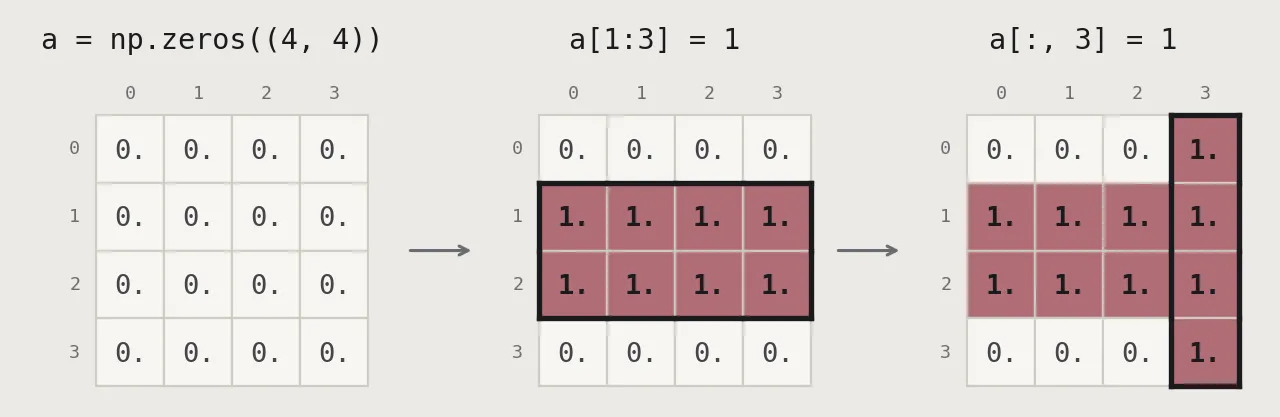
Changing shape
np.transpose
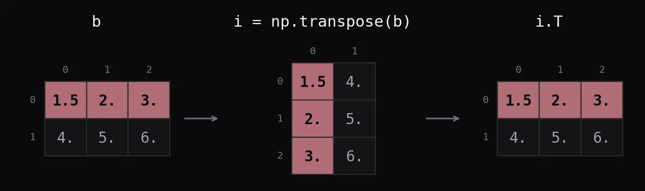
Swaps the axes, so row 0 becomes column 0. .T is the short form, and transposing twice gives b back.
i = np.transpose(b)
i.T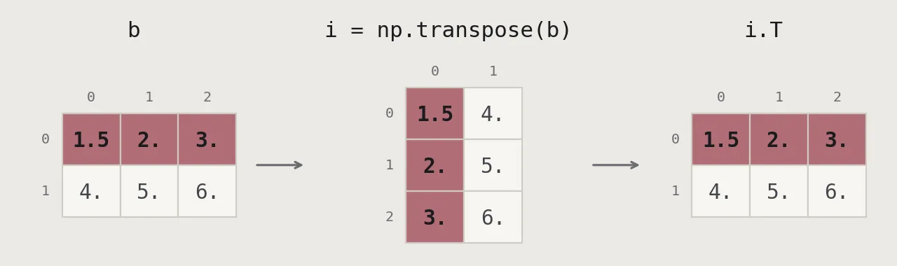
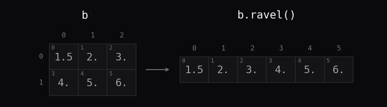
b.ravel
Flattens to 1D in row order.
b.ravel()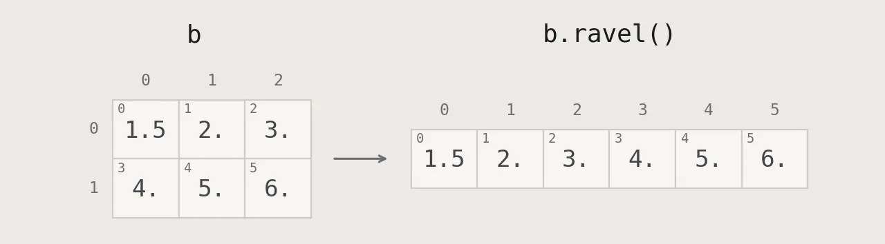
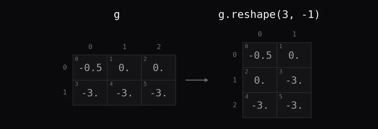
g.reshape
The same data in a new shape; the elements keep their order. -1 means ‘work this size out’. The sheet writes -2, which NumPy happens to accept, but -1 is the documented value.
g.reshape(3, -1)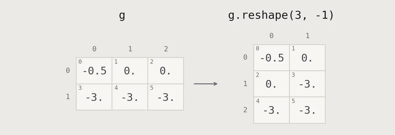
resize
The sheet calls h.resize on a view, which raises ValueError: cannot resize this array: it does not own its data. On an array that owns its data, the method works in place and pads with zeros. The function np.resize returns a new array and repeats the data instead.
h = b.copy()
h.resize((2, 6))
np.resize(b, (2, 6))

Adding and removing elements
np.append
Flattens both arrays and joins them into a new 1D array. Pass axis= to keep the shape.
np.append(a, b)

np.insert
Inserts 5 before index 1 and returns a new array. A NumPy array never grows in place.
np.insert(a, 1, 5)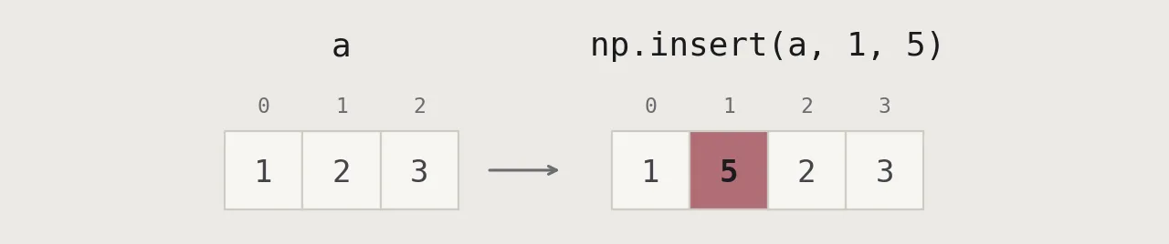

np.delete
Removes index 1 and returns a new array.
np.delete(a, [1])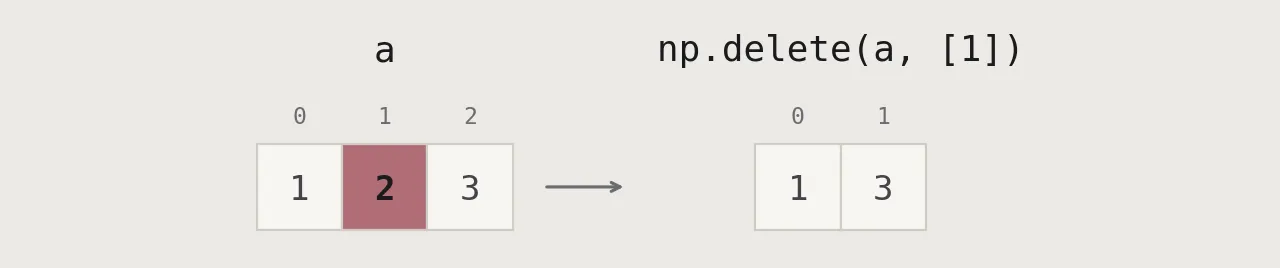

Combining arrays
np.concatenate
Joins arrays along an axis they already have.
np.concatenate((a, d), axis=0)

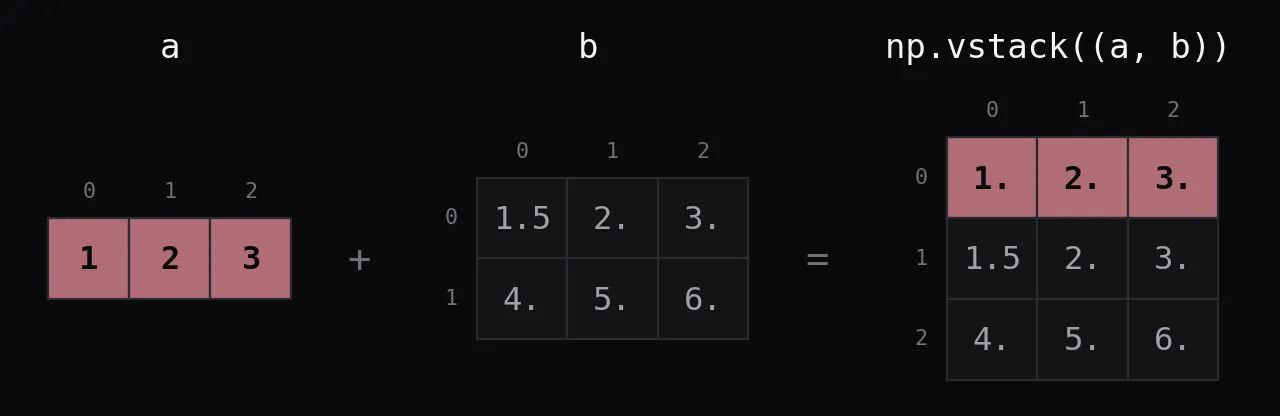
np.vstack
Stacks rows: a becomes the first row and b’s rows follow.
np.vstack((a, b))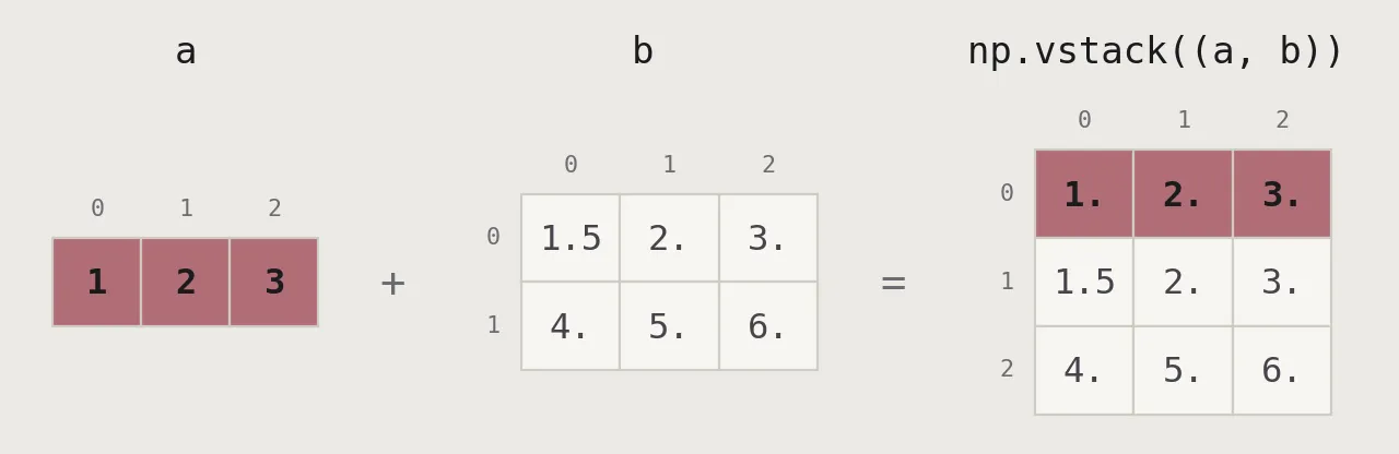
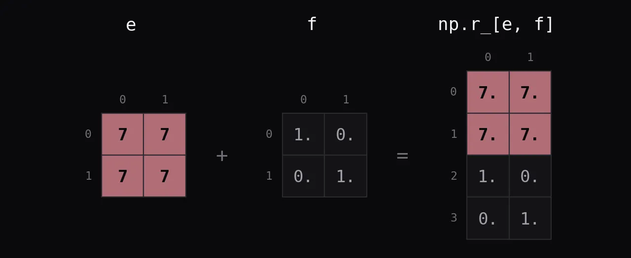
np.r_
Index-style shorthand that concatenates along axis 0, here the same as np.vstack((e, f)).
np.r_[e, f]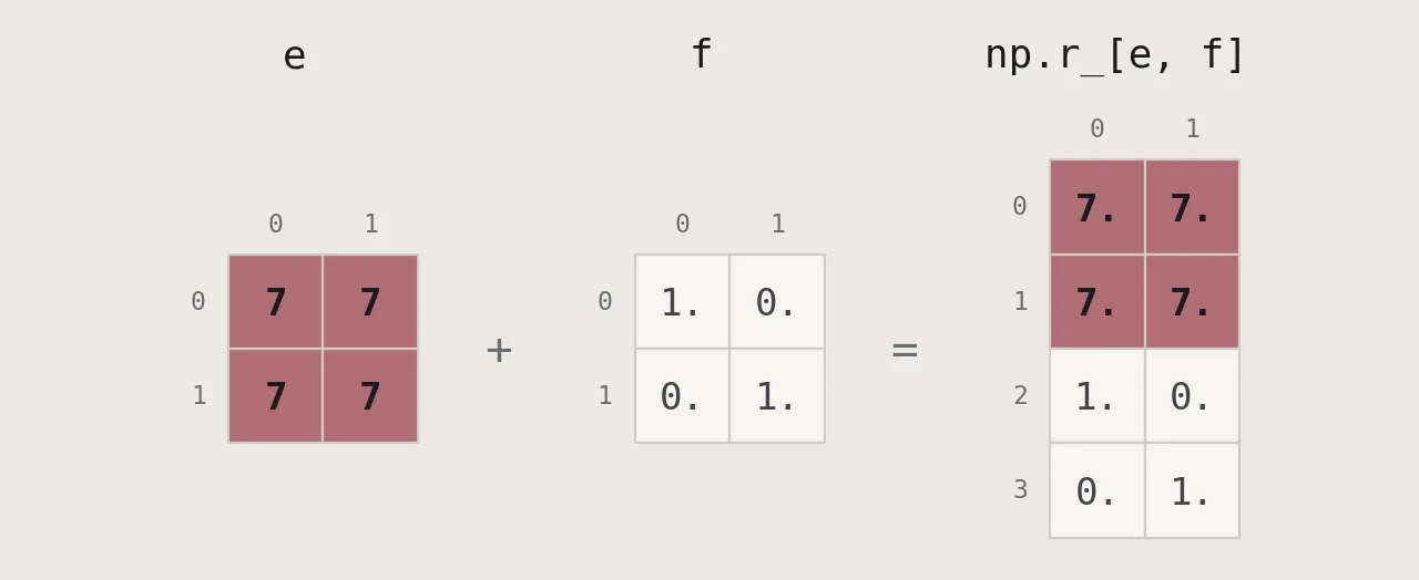
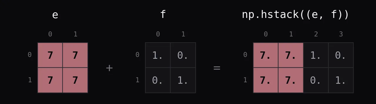
np.hstack
Joins side by side, along axis 1.
np.hstack((e, f))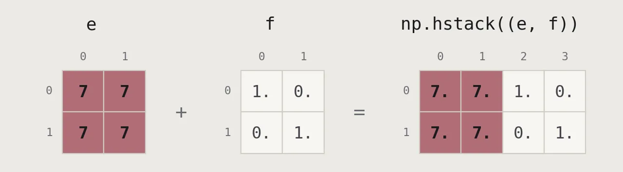
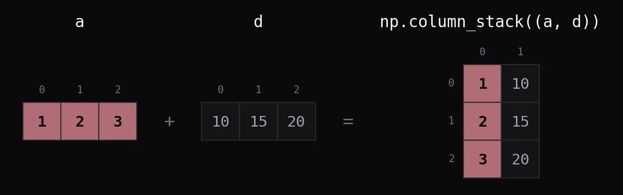
np.column_stack
Turns 1D arrays into columns. np.c_[a, d] gives the same result.
np.column_stack((a, d))
np.c_[a, d]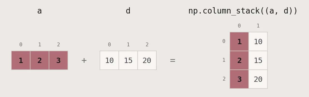
Splitting arrays
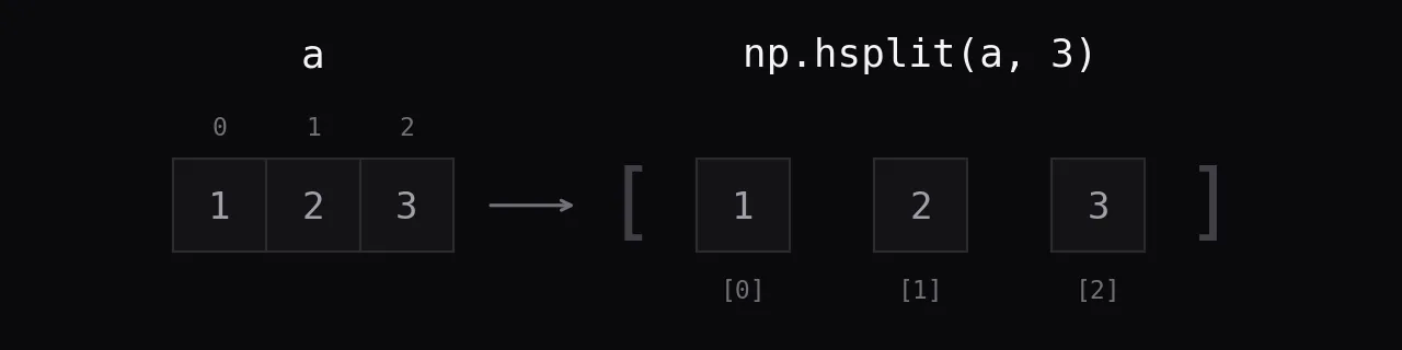
np.hsplit
Splits into 3 equal pieces along axis 1, which for a 1D array is its only axis. The result is a list of arrays.
np.hsplit(a, 3)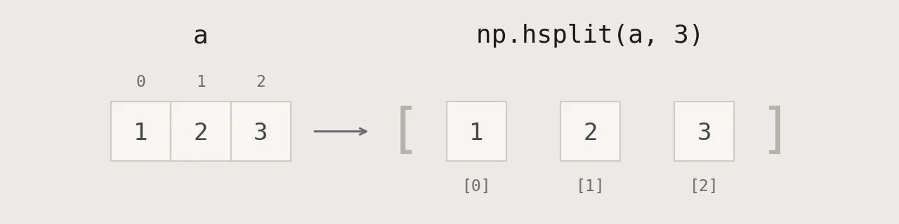
np.vsplit
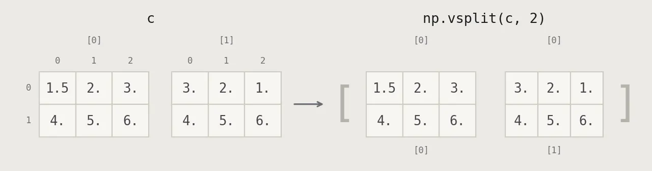
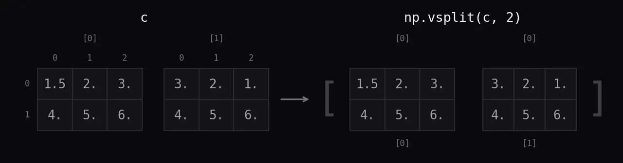
Splits along axis 0 into 2 pieces, here the two blocks of c. The values the sheet prints for this line are wrong; the picture shows the real ones.
np.vsplit(c, 2)